The Distance Geometry Problem (DGP) asks whether a simple weighted undirected graph G=(V,E,d) can be realized in a K-dimensional space so that the distance between each pair of realized vertices u and v is the same as the weight d(u,v) assigned to the edge {u,v}, when available. The distance function d generally associates an interval [lb(u,v),ub(u,v)] to every edge {u,v} of E. The range of the interval corresponds to the uncertainty on the actual value of the distance: when the interval is degenerate, i.e. lb(u,v) = ub(u,v), then there can be two different situations: either the distance is exact (i.e. provided with high precision), or the level of uncertainty on the distance is not a priori known, so that only an approximated value is provided. Notice that the embedding space is Euclidean in several real-life applications. The DGP is NP-hard, and in the last years, together with several other colleagues, we have been working on the different facets of this problem.

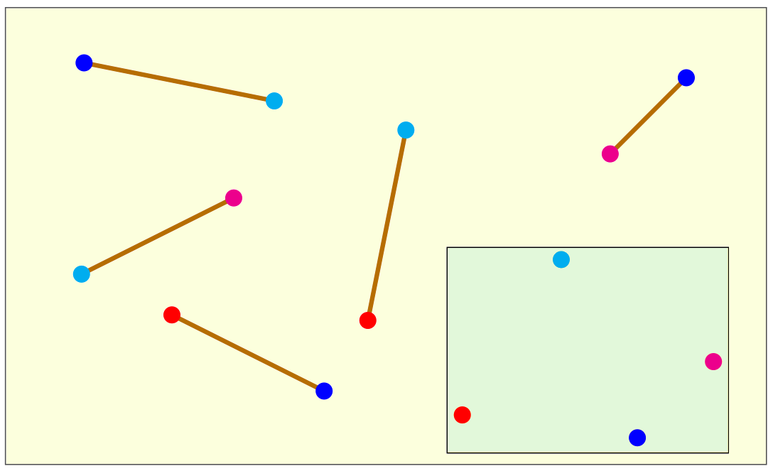
   The drawing below depicts the input and the output of a DGP instance in the 2-dimensional Euclidean space.

The sticks are the edges of the graph G representing the DGP instance. Their length corresponds to the weight on the edges, which is the numerical value of the distance. In this example, there are 5 edges in G connecting 4 vertices in 5 different ways. Each vertex is marked in the drawing with a different color. In the hypothesis the sticks are rigid (i.e., they are not elastic), and hence the corresponding distances are exact, then the vertex positions shown in the small box give one of the possible solutions to the DGP on the Euclidean plane. Other possible solutions can be obtained by translating, rotating or (partially, in some cases) reflecting this given solution. One way to perceive the complexity of the DGP is to look at the set of sticks when disconnected from each other, and try to figure out the geometric figures associated to the DGP solutions.

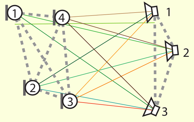
   The DGP has several important applications. One classical DGP application arises in biology: experiments of Nuclear Magnetic Resonance (NMR) are able to find estimates of some distances between atom pairs in molecules, so that the solution to the corresponding DGP allows for finding molecular conformations. Molecules can be represented in the three-dimensional Euclidean space. Other applications of the DGP include the sensor network localization problem (in dimension 2), acoustic networks and graph drawing (generally in dimensions 2 or 3), clock synchronization (in dimension 1), and multi-dimensional scaling (in any dimensions).

The drawings above show two of the mentioned applications. On the left-hand side, the conformation of the protein having code 1mbn on the Protein Data Bank; on the right-hand side, an example of acoustic network (picture extracted from this article).

   The discretization of the DGP can be performed when the graph G satisfies some particular assumptions. These assumptions ensure that every vertex v of the graph has at least K adjacent predecessors, which can serve as a reference for computing candidate positions for the vertex (where K is the dimension of the embedding space). The identification of the feasible positions for a given vertex are computed by intersecting the K Euclidean objects related to the K adjacent predecessors of the vertex. These Euclidean objects are points in dimension 1, circles in dimension 2, spheres in dimension 3, and hyper-spheres in any other dimension. Under the discretization assumptions, the intersection of these Euclidean objects always gives a discrete and finite number of feasible positions.

   In order to fix the coordinate space and avoid that the obtained conformations can "float" in the space, it is also required that the first K vertices form a clique. An example is given below for K = 2. The first two vertices (forming the clique) can be fixed in two unique positions. For all other vertices, even if more than one position can be assigned to them, the total number of positions per vertex remains finite.

In this small example, the vertices labeled from 3 to 5 admit more than one possible position in the 2-dimensional space. In the drawing, the circle defined by the reference vertex with lowest rank is explicitly shown, while only small marks, indicating the intersection points, are given for the second (having higher rank) reference vertex.

   The solutions to this small instance are given by the set of paths connecting the vertex 1 with any of the found positions for the vertex 5. The drawing shows that the solution set has the structure of a tree, which grows exponentially with the number of involved vertices. This is consequence of the fact that the DGP is an NP-hard problem. Moreover, the search tree is symmetric: in this example, the line going through every pair of reference vertices defines a symmetric axis, such that all distances (between any of the reference vertices and any of the "subsequent" vertices) that are satisfied (or not) by the solutions on the left-hand side of the symmetry axis are also satisfied (or not) by the solutions on the right-hand side of the symmetry axis.

   In this example, the solution set corresponds to the entire search tree. However, when additional distances are available, they can be used for selecting a subset of solutions from the search tree. In practice, the idea is to construct the search tree step by step while performing a depth-first tree search where the additional distance information (used to perform these selections) is used as soon as the vertex positions necessary for the verification are computed. In this way, some branches of the search tree are not generated at all, because it is known in advance that they contain infeasible solutions. In this case, we say that the branches of the tree are "pruned", and the distances used to perform this operation are generally referred to as "pruning distances". The general algorithmic framework implementing this idea is for this reason named the branch-and-prune (BP) algorithm.

   The DGP that satisfies the discretization assumptions is called the Discretizable DGP (DDGP). Remark that the discretization does not change the problem complexity, which remains NP-hard.

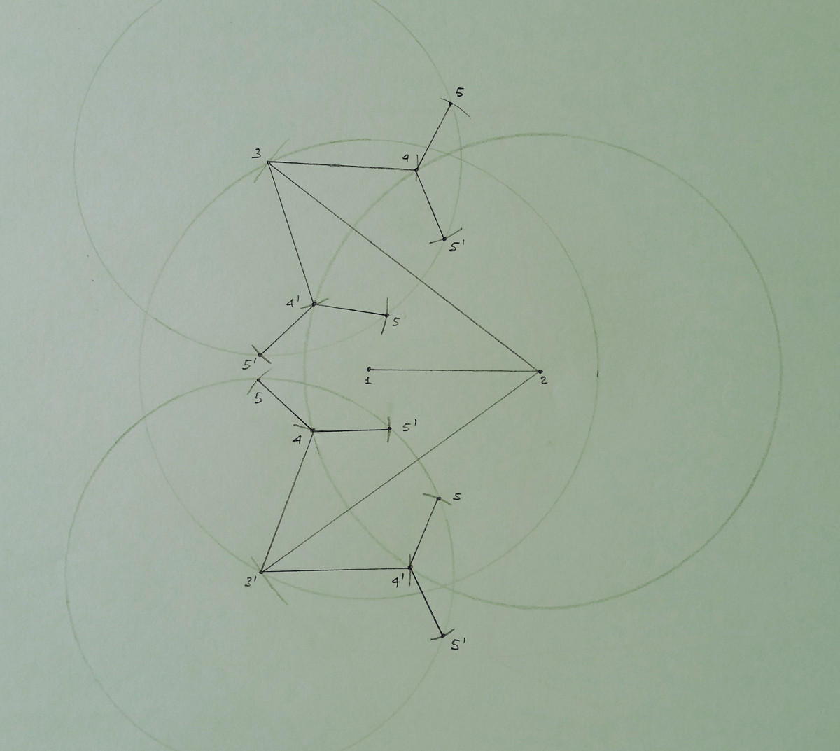
   In the example given above, the graph G, with the vertex ordering specified by the numerical labels, actually satisfies an additional assumption: for every vertex v, the reference vertices are its two immediately preceding vertices (for example, the reference vertices for 5 are 3 and 4). This assumption is known under the name of "consecutivity assumption". However, this assumption is not strictly necessary to perform the discretization of the DGP. The example below shows in fact another example where the consecutivity assumption is not satisfied: both vertices 4 and 5 have as reference vertices the vertex 2 and the vertex 3.

In the figure above, the circles and the marks are drawn by following the same criteria indicated for the previous drawing. This example basically shows that, when the consecutivity assumption is not satisfied, the search domain is not necessarily a binary tree (even if it can be approximated by a binary tree, as it was previously done in many publications), and the reference vertices for different vertices can form a common symmetry axis. In this example, it is also supposed, for simplicity, that the distance between the vertex 2 and 4 coincide with the distance between 2 and 5 (the positions for both 4 and 5 lie on a common circle).

   As remarked above, the pruning distances allow us to select the branches of the search tree that contain feasible DGP solutions. When the distances are exact and their numerical value is very precise, the presence of a pruning distance from the vertex u to the vertex v, in this order in the search tree, makes it possible to reduce the total number of vertex positions computed for v to the same number of positions found for u. This is a very important property of DDGPs, because it allows us to estimate in advance the number of solutions that we can expect to find in the search tree.

   The paradoxical DGP instance is a particular DDGP case where this property seems to suggest, at the same time, that the instance is simple, as well as hard. This DGP instance satisfies the discretization assumptions but it contains only one extra distance playing the role of pruning distance: this is the distance between the very first and the very last vertex of the graph G. We can therefore say that this instance is simple because, for the property mentioned above, we know in advance that its search space contains only two symmetric solutions (symmetric w.r.t the hyper-plane defined by an embedding of the initial clique). But we can also say that this instance is hard because, in order to identify these two symmetric solutions, the entire search domain, up to the last but first layer, needs to be constructed. No branch selections can be performed before reaching the very last layer of the search tree.

   We are currently working on an experimental technique in Optical Computing for an efficient solution of the paradoxical instances of the DGP. More details about this research direction are given in the talk below, which is part of our mini-symposium at Fields Institute, and available on YouTube's Fields channel.

   In order to deal with real-life data, where distances are generally imprecise and often represented by intervals having relatively large ranges, it is required that at least K-1 reference distances can be considered as "exact" (meaning by "exact" that lb(u,v) = ub(u,v) and the approximated distance value is not affected by an error that is higher than the predefined tolerance error). As a consequence, the Euclidean objects involved in the intersections (performed to determine the feasible points for a given vertex v) are not always (hyper-)spheres, but rather (hyper-)spherical shells may actually be involved in the intersection in presence of an interval distance.

   In these hypotheses, the intersection does not provide a finite number of feasible points, but rather a continuous object in dimension 1 (a set of arcs delimited on the circle defined by the K -1 spheres). One of the initial employed strategies to deal with interval distances consisted in discretizing these arcs, by simply extracting equidistant sample points from each arc obtained with the intersections. However, it is now known that this strategy can introduce an important error capable to propagate along the search domain, and to completely spoil the computations. Therefore, more recently, we have proposed a coarse-grained representation for the solutions of the discrete search domain of DDGPs. The BP algorithm implementing this coarse-grained representation is actually the very first implementation that can efficiently handle the DGP instances containing interval distances.

   Recent works have been focusing on the dynamical character of some DGP applications. To represent a dynamical DGP instance, we use a graph G having a special vertex set V × T, where V is a set of objects (the static vertices of the classical problem), while T represents the time as a sequence of discrete steps. The dynamical DGP (dynDGP) was introduced in the talk reported below in 2017.

Some animations obtained via dynamical DGPs can be viewed on my dynDGP animations page.

   In recent studies, the dynDGP was employed for tackling some typical problems in computer graphics, such as the "human motion adaptation problem". This talk, presented during our mini-symposium at Fields Institute, gives an overview on these initial studies.

   MD-jeep is an implementation of the BP algorithm for DDGPs, which is available on GitHub since the release 0.3.0, where the software tool was extended for solving instances containing interval distances (see section above about the coarse-grained representation). Differently from other software tools for the DGP, MD-jeep is able to enumerate the entire solution set for a given instance. This is trivially done with instances consisting of only exact distances by performing the entire exploration of the search tree (which is in practice possible when a sufficient number of pruning distances is available). In order to do the same for instances containing interval distances, the resolution parameter was recently introduced in MD-jeep. This parameter allows us to select solutions from a (local) continuous set of feasible solutions.

   Meta-heuristics are widely employed in optimization. My first experience with meta-heuristics dates back to my PhD in Italy, where I was working on a geometric model for the simulation of protein conformations. This model leads to the definition of a global optimization problem, whose solutions represent geometrically "well-shaped" conformations for proteins, that we were used to obtain by executing a simple Simulated Annealing (SA). The permutations implemented in our SA implementations were particularly inspired by the geometric nature of the considered problem.

   A few years later, I took part of the development of a novel meta-heuristic framework which is inspired by the behavior of a monkey climbing trees of solutions with the aim of finding good-quality solution approximations. We named this method the Monkey Search.

A monkey can in fact survive in a forest because it is able to focus its food researches where it has already found food. The trees the monkey explores contain solutions to the optimization problem to be solved, and branches of the tree represent perturbations able to transform one solution into another. At each step, the monkey chooses the branches to climb by applying a random mechanism, which is based on the objective function values of the new corresponding solutions. Notice that, rather than a completely new meta-heuristic approach for global optimization, the Monkey Search can be considered as a general framework describing the monkey behavior, where other ideas and strategies for global optimization are also employed.

   In the context of data mining (see below), we have been working on techniques for supervised biclustering. We proposed a bilevel reformulation of the associated optimization problem, where the inner problem is linear, and its solutions are also solutions to the original problem. In order to solve the bilevel problem, we have developed an algorithm that performs a Variable Neighborhood Search (VNS) in the space defined by the outer problem, while the inner problem is solved exactly by linear programming at each iteration of the VNS.

   More recently, we proposed the environment as a new general concept in meta-heuristics. As of today, we have tested this novel idea in conjunction with only one meta-heuristic: the Ant Colony Optimization (ACO). In ACO, artificial ants move in a mathematical space by following the pheromone trails left by ants having previously explored the same region of the search space. Our environment perturbs the perception of the pheromone, for ants to avoid to get trapped at local optima of the considered problem. In a recent work, we used our ACO with environmental changes for inter-criteria analysis. Work is in progress for a theoretical study for this new meta-heuristic concept, as well as for testing this novel idea with other meta-heuristics.

   Data mining consists in extracting previously unknown, potentially useful and reliable patterns from a given set of data. In collaboration with Panos Pardalos and Petraq Papajorgji, we wrote a textbook describing the most common data mining techniques, by paying a particular attention to those used in the agricultural field. One interesting example is the problem of predicting, by using the data obtained from the very first stages of the fermentation, the wine fermentations that are likely to be problematic, in order for the enologist to take actions in advance to avoid spoiling part of the production.

   After the publication of the book, we worked on supervised biclustering techniques for classification. Given a set of data, biclustering aims at finding simultaneous partitions in biclusters of its samples and of the features which are used for representing the samples. Consistent biclusterings can be exploited for performing supervised classifications, as well as for solving feature selection problems. The problem of identifying a consistent biclustering can be formulated as a 0-1 linear fractional optimization problem, which is NP-hard. We worked on a bilevel reformulation of this optimization problem, and on a heuristic (see above) which is based on the bilevel reformulation.

   In the different problems introduced above, the main considered application (at least in my publications) is the one of analyzing or identifying the three-dimensional conformation of protein conformations. Why all this interest?

C.M. Dobson, A. Sali and M. Karplus wrote: An understand of folding is important for the analysis of many events involved in cellular regulation, the design of proteins with novel functions, the utilization of sequence information from the various genome projects, and the development of novel therapeutic strategies for treating or preventing debilitating human diseases that are associated with the failure of proteins to fold correctly.

   Here's below a brief description of protein conformations that I wrote at the very beginning of my research on this topic (in other words, this is a description from a non-specialist, but that the mathematician or computer scientist may easily follow).

Proteins are heteropolymers. They are formed by smaller molecules called amino acids, that are bonded together to form a sort of "chain". Living organisms contain plenty of proteins, which perform several functions of vital importance. Each amino acid along the protein chain contains a Carbon atom called C_α, which is chemically bonded to three different aggregates of atoms. Two of these aggregates are common to each amino acid: the amino group (NH₂) and the carboxyl group (COOH). Only one aggregate of atoms makes each amino acid different from one another: the so-called side chain R. Only 20 amino acids are involved into the protein synthesis. These molecules are under genetic control: the amino acid sequence of a protein is contained into the corresponding gene of the DNA molecule. The three-dimensional conformation of a protein molecule is of great interest, because it defines its dynamics in the cell, and therefore its function.

Different properties of the side chains allow for classifying the amino acids on the basis of their features. A very important feature of the amino acids is the polarity of their side chains R. A side chain is polar if it has a global or local electric charge. There is an attraction between positive and negative charged molecules and there is repulsion between molecules with the same charge. Since the protein solvent, i.e. water, is polar and globally uncharged, there is attraction between the water molecules and the polar R groups. It follows that the amino acids having a polar side chain are hydrophilic, because they tend to interact with the solvent. Other amino acids are buried inside the protein because of the hydrophilic amino acid behavior. Therefore, they are called hydrophobic. This feature of the amino acids plays a fundamental role in the stabilization of protein molecules. The attractive and repulsive van der Waals forces are important as well. They can be modeled, for example, by the Lennard Jones potential (see below). This page provides additional information about amino acids.

Each amino acid of the protein chain is bonded to the previous and the successive amino acid through a peptide bond. More precisely, the carboxyl group of the i^th amino acid is bonded to the amino group of the (i+1)^th amino acid, i.e. a covalent bond keeps bonded the C atom of the first group and the N atom of the second one. The peptide bond is strong enough to force every atom between two consecutive C_α atoms on the same plane. Therefore, the movement possibilities of the amino acids on the chain are strongly constrained.

   Finding the ground state conformations of clusters of molecules is one of the most difficult global optimization problems. Such clusters are regulated by potential energy functions, such as the Lennard Jones and the Morse potential energy (also involved in the identification of protein conformations, see above). The Lennard Jones potential is very simple but sufficiently accurate for noble gas, and it also provides approximations for structures of nickel and gold. The Morse potential has a parameter which determines the width of the potential well; Morse clusters show a wide variety of structural behaviors in function of this parameter. Both potential functions have several local minima in which methods for optimization may get stuck at. For instance, a Lennard Jones cluster formed by 13 atoms has about 1000 local minima, and the number of local minima increases exponentially with the size of the cluster. The Lennard Jones and Morse optimal clusters usually have particular geometric motifs, which can be exploited during the optimization process. The Cambridge Cluster Database contains experimentally obtained clusters. Some of them may just be local minima: the database is open to newly generated clusters having a lower energy function value.

The drawings above that I made with pencil and compass are not meant to be precise but they intend only to visually show the main ideas behind the discretization of DGPs. The idea to make such drawings came into my mind quite recently, while I was helping my kid with his homeworks...